Corporate leaders frequently have to make decisions on whether to sanction investment in innovations or reject the investment request. Generally, the most common and widely used metric for capital budgeting and decision making is the Net Present Value, aided by Discounted Cash Flow. This metric is however only fairly accurate when dealing with innovations with a high degree of certainty, which is typically aligned with incremental and efficiency innovations. However, when leaders are faced with innovations with high uncertainty (disruptive, semi-radical or radical innovation) they often rely on the same metric, which can result in two types of decision making errors. These are errors of false positive or false negative. False positive is when an innovation opportunity is deemed as economically viable and thus pursued, but in reality, it is unviable. False negative is when an innovation opportunity is deemed as economically unviable and thus rejected, but in reality, it actually has positive economic returns. These potential problems emanate from the very nature and attributes of DCF and NPV methodology. The DCF & NPV approach is designed as a static methodology, which in addition to the capital investment outlay, considers estimated revenues and costs for each year that the venture will be operating and then applies a risk adjusted discount rate to calculate the NPV. This methodology implicitly assumes that the estimated yearly cash flows (which are educated guesses at best) are fixed, with the framework having no means of allowing for uncertainty in those values. This is not so much of a problem for opportunities where there is high certainty and accuracy in these numbers. However, with disruptive and radical ideas or other opportunities with volatility, the method comes up short due to its inability to be flexible and value the inherent uncertainty or risk. So how do innovation leaders tackle this problem? The answer lies in Real Options Valuation.
Despite their ability to uncover hidden value in innovation projects, adoption of Real Options Valuation remain low within innovation, capital budgeting and CFO circles. Low adoption is perhaps due to lack of familiarity and sometimes the complexity of the techniques involved. Considering the significant impact real options can have for organisations, from both the upside and downside scenarios, we aim to help capital budgeting practitioners (including those sanctioning innovation opportunities) to better understand real options. In this article, we will introduce real options with a much more granular approach and with examples showing step by step methodology on how to evaluate the real options in different scenarios. We will also adopt a much easier to understand, albeit slightly more rigorous binomial model instead of the more complex Black and Scholes replicating portfolio model.
NPV and Real Options
Whilst the traditional NPV approach ignores the value of risk, uncertainty and flexibility, by taking a single focused now or never, go or no-go approach, Real Options Valuation methodology considers risks and uncertainty as opportunities and allows the organisation to exploit the upside whilst rejecting the downside. As such, real option methodology allows decision makers to structure the right innovation opportunity as an option, one that the owner can either decide to exercise within a certain period of time (option life), if the risks and uncertainty evolve positively and shows the opportunity to be “in the money”, or the owner can chose to walk away from it, if the conditions evolve negatively and shows the opportunity to be “out of the money”.
With real options valuation, innovation leaders can value their opportunities, where applicable, using one of three options approach. These are option to delay, option to expand and option to abandon.
Option to Delay
This is a real option valuation that looks to understand the possible downside and upside values of an opportunity over a set period of time (option life). If the positive outcome results in economic viability, the organisation will wait (option to delay) for the right time before exercising that option. The uncertainty in option to delay is typically driven (and calculated) by volatility of revenues (price or market size) based on the assumption that more often than not costs can be more accurately estimated than what an acceptable selling price, or what the market size (demand), will be. Typical opportunities that represents option to delay are patent protected ideas, undeveloped natural resources such as in an oil reservoir and radical ideas that very few organisations are competing in during the life of the option. In effect option to delay are most appropriate when there is a degree of exclusivity to the market opportunity for a specific period of time (option life). However, they can still be applied in other scenarios with less exclusivity.
Option to Expand
This is a real option valuation where before the organisation takes an initial opportunity (sometimes, even as a loss-making strategic investment), it values the future opportunity that will be made possible by the initial investment and thus position itself to be able to exercise future option to expand and turn the overall investment into an economically viable venture. Imagine the case of Jeff Bezos and Amazon, where the initial investment was loss making for many years, but that initial investment position gave Amazon the option to further expand in the e-commerce space. An option that Amazon did exercise. We are not affirming that Jeff Bezos used a real options valuation approach. However, the evolution of Amazon is a classic option to expand scenario.
Option to Abandon
This is a real option valuation where an organisation considers investing in an opportunity where there is no option (or further option) to delay, but considers the residual value of the opportunity in the downside scenario where there might be a need to stop the project and walk away. Such an option will be characterised by either a residual value of assets that can be re-couped or perhaps a buyout offer in a joint venture or partnership, which must be exercised within a certain period, which is the life of the option.
Parallels between financial options and real options
To better understand innovation as real options, a parallel can be drawn to more familiar financial options as shown below
In stock market investing, we can compare two different investment approaches, (i) Investor A takes a long position of £10,000 (perhaps based on technical analysis) in the shares of Qubixz Limited. (ii) Investor B buys a 12 month call option for £100 (as an example) to purchase 1000 Qubixz shares at £10/share.
Investor A has taken a full investment position and is equally exposed to both the upside and downside of Qubixz’s share price and can lose the entire £10,000. Investor B on the other hand is fully exposed to the upside but has limited his downside risk to just £100 by taking out a call option. Investor B has effectively taken an option to delay investment, which can be exercised if Qubixz share price rises and the option is “in the money” or can walk away if share price falls and the option is “out of the money”. The price paid for the call option is the maximum downside that can be experienced.
We can compare the two Qubixz investment approaches to a static NPV vs Real Option innovation decision making approaches, as shown below with the false positive scenario
Real Options under False Positive Scenario
(i) Company A, based on NPV analysis of £10m, invests in a new radical product with an upfront capital investment of £100m (ii) Company B carries out the same NPV analysis which also shows an NPV of £10m at £100m investment. However, due to the high volatility of expected cash flows (uncertainty and risk) attached to this radical innovation, Company B decides to carry out a real options valuation with an option life of 5 years and determines that based on the volatility, by the 5th year, the present value of £110m can vary from as low as £24m to as high as £500m. Based on this wide-ranging possibilities, Company B takes an option to delay investment. Over the next five years, Company B continues to carry out market research, prototyping and further product development at a total cost of £0.5m, only to find out that the innovation is not economically viable and will in fact result in a value of only £24m. Based on this Company B walks away from the investment and loses £0.5m, which is effectively the price of the option (equivalent to £100 in the Qubixz Limited share option comparison). Company A on the other hand stand to lose as much as £76m (£24m - £100m) by not taking a real options approach.
The above example is based on a false positive analysis. Below we also take a look at a false negative scenario
Real Options under False Negative Scenario
(i) Company A, based on NPV analysis of -£5m, decides not to invest a new radical product with an upfront capital investment of £100m (ii) Company B carries out the same NPV analysis which also shows an NPV of -£5m at £100m investment. However, due to the high volatility of expected cash flows (uncertainty and risk) attached to this radical innovation, Company B decides to carry out a real options valuation with an option life of 5 years and determines that based on the volatility, the present value of £95m can vary from as low as £18m to as high as £500m over the life of the option. Based on this wide-ranging possibilities, instead of walking away, Company B takes an option to delay investment. Over the next five years, Company B continues to carry out market research, prototyping and further product development at a total cost of £0.5m, only to find out that the innovation is indeed economically viable and will in fact result in a future value of £500m. Based on this, Company B exercise the option to delay and invest, thus capturing value from the innovation whilst Company A completely misses out on this opportunity due to its false negative error caused by a static NPV approach.
As shown in these sterilised examples, real options mandate managers to look beyond estimated present value of ideas and consider the range of future outcomes. To get an understanding of what drives this future outcomes we need to examine the characteristics of real options valuation and what a real options valuation entails.
Characteristics of Real Options Valuation
Real options emerged out of the financial option pricing industry and whilst financial option pricing as determined by Black and Scholes uses a potentially complicated replicating portfolio approach (a portfolio consisting of the underlying asset and a risk free asset that has the same cash flow as the option being valued) to come up with the option value, we will adopt the much simpler binomial model (with event tree) for valuing innovation options.
It is also worth noting that real options valuation approach is not an alternative to the traditional NPV approach, it is an augmentation. Decision makers need to first carry out a DCF & NPV calculation before proceeding to real options valuation – don’t throw out your NPV spreadsheet just yet. As a final outcome, the real options value is added to the NPV in order to determine the overall value, which includes the upside of uncertainty and risk. As such, an expanded NPV is calculated for the opportunity as below
Expanded NPV = Static NPV + Option Value
We will now look at the determinants of real options valuation.
Determinants of Real Options
There are six levers that impact the value of an option as outlined below
Value of Asset (V0). The starting point of building the binomial tree and determining the value of an option is to estimate a value for the underlying asset. For an innovation opportunity, the value of the underlying is determined as the Present Value (PV) of all post tax cash flows. This is the underlying valuation principle in finance that states that the value of any asset is the sum of the present values of all future cash flows.
Value of Investment (I). This is the present value of the capital investment required in the opportunity. This is sometime referred to as the exercise or strike price.
Life of Option (t). This is the period in which the opportunity remains valid as an option and the go / no-go decision must be taken within that period. Innovation practitioners must determine a realistic time frame within which the opportunity remains largely uncontested by competitors and thus represents the option life. A typical example will be a patent that lasts 10 years. The option life in this case is 10 years. For a radical (new) innovation without patent, the owner might take a view that the opportunity will be largely uncontested for 3 or 5 years or may be longer.
Volatility of Cash Flows (s). Volatility is what gives the underlying asset the tendency to have potential downside and upside from the present value (Value of Asset, V0) estimate. Volatility of cash flow is perhaps the most difficult lever to determine due to the fact that a radical innovation opportunity does not have any empirical cash flow data upon which distribution of cash flows can be determined. As such there are two recommended approaches; (i) experiential managerial estimates of minimum and maximum deviation from the estimated cash flow, (ii) Related industry standard deviation data of firms’ value.
Option Discount Rate (r). This is the risk-free interest rate corresponding to the option life. This value is typically equivalent to the riskless government treasury rate over the life of the option. This rate is used to discount the future payoffs determined for the asset and ultimately calculate (or arrive at) the option value. This is the minimum rate that investors can expect on their investment on the project.
Cost of Option (c). This is the cost of keeping an option open and it is typically estimated on a yearly basis. The cost of keeping an option open is equivalent to the yearly fractional loss in the value of the underlying asset for every year that the option is not exercised. As an example if the value of the underlying asset (V0) is £100m for a 20 year project life, the yearly cost of keeping the option open will be (100/20). In financial options, this is equivalent to buying a call option on a stock and missing out on the dividends until such time that the option is exercised.
These levers form the basis of determining option values and are used in building the binomial model event tree that provides the final option value.
The Binomial Model
The binomial model is based on the premise that in any given time interval during the option life, the value of the underlying asset can either go up by a certain factor (u) or go down by a certain factor (d). This is shown in the below illustration for a 2 year option with 1 year intervals

The factors u and d are functions of volatility and time. Using the volatility and the option time interval (dt, years), – which is the option life in years divided by the number of intervals (two intervals shown above) - the factors u and d can be calculated as shown below.
u = exp (s*√dt)
d = 1/u
The formulae for u and d are determined on the basis that variation in value will typically follow a continuous normal distribution.
The model also determines that the upward movement (u) is subject to a risk neutral probability pu, whilst the downward movement is subject to risk neutral probability of pd. These probabilities are calculated as
pu = [exp(r*dt)-d]/[u – d]
pd = 1 - pu
These probabilities, along with the risk free interest rate are used to discount the future pay-off back from the point of the option exercise to the present.
We will now work through some examples to show how real option valuation works in practice
Option to Delay Case Study
Qubixz UK Limited is developing a new wearable technology that enables people to communicate without mobile phones. This is a radical innovation that Qubixz has patented for 10 years and is planning to release the product into the market. Based on current analysis, the following data has been generated
Cost of globally launching the new wearable, I = £ 2.5 billion
PV of 20 year post tax cash flow if product is released now, V0= £ 2.3 billion
Patent Life (option Life), t = 10 years
Risk free rate, r = 2% (10 year UK govt. treasury rate)
Volatility expected in value, s = 0.4 (This is SD in firm value in tech industry)
Cost of option per year, c = (2.3/20) = £0.115 billion / year
We will now take a stepwise approach to valuing the option to delay this investment and the resulting expanded NPV
Step 1. Traditional NPV Calculation
First we look at the static NPV of this opportunity, which considers investing in the project today based on Cost of Investment and PV of cash flows. We get an NPV of -£ 0.2 billion (£2.3b - £2.5b), thus making this a non-viable project (today) from the NPV point of view.
Step 2. Build the Event Tree of Future Values
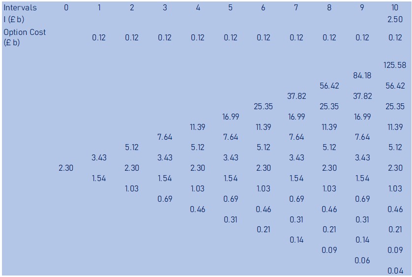
To assess this opportunity as an option that Qubixz may choose to exercise at the 10 year expiration and see if there is a chance that the option value will result in opportunity being economically viable, we need to build an event tree of future values.
To do this, based on the volatility we will determine how the underlying asset of £2.3 billion may grow or diminish over the next 10 years. For this we need to calculate the u and d factors. Using yearly intervals (10 intervals), we calculate as follows
u = exp (s*√dt) = exp (0.4*sqrt (10/10)) = 1.492
d = 1/1.492 = 0.670
Based on the PV of cash flow and the u and d factors, we can now build our binomial event tree of all the possible future values of the opportunity over the next 10 years. As an example, the first up value and down value are calculated as
2.3*1.492 = £3.43 billion
2.3*0.670 = £1.54 billion
Possible future values (V, £ billions) of Qubixz Limited’s wearable is as shown in the binomial tree below
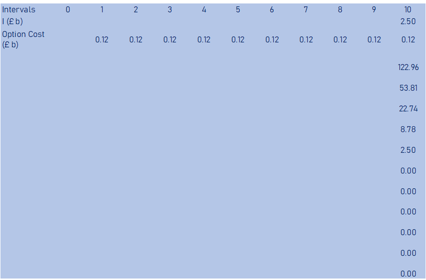
Step 3. Determine the Pay-off at Option Exercise
From the future values (V), we will now calculate all the possible pay-offs during option exercise at the end of the option life (year 10). The pay-off will be the Maximum of V – I – c or 0. This is sometimes written as Max (V – I – c, 0).
As an example, V at the top right hand corner of the tree, which shows that if the value of the asset went up every year it will reach £125.58 billion, the pay-off will be
125.58 – 2.5 – 0.115 = £ 122.96 billion
Whilst the at the bottom right hand corner of the tree, which shows that if the value of the asset went down every year it will fall to £ 0.04 billion, the pay-off will be
0.04 – 2.5 – 0.115 = £ 0
The implication here is that, for future values that have a positive pay-off, Qubixz Limited will choose to exercise this option and launch its wearable device and for future values that have a negative pay-off, Qubixz Limited will walk away, effectively making the pay-off zero.
Using this Max pay-off calculation formulae, we will calculate the pay-off for all future values V at the final year of the option, which is year 10 in this case. The result is shown in the binomial tree year 10 pay-offs table below.
The next step is to then discount these pay-offs back to time zero, using the risk free rate (minimum rate of return).
4. Discount Pay-offs Back to Year 0
Once we determine all pay-off values at year 10 where Qubixz Limited may choose to exercise the option of launching its wearable technology, we will now discount all the pay-offs back to the present using the risk free discount rate and probabilities of both u and d movements.
pu = [exp(0.02*1)-0.67]/[1.492-0.67] = 0.426
pd = 1 - pu = 0.574
The discounting will be done one year at a time, whilst building the binomial tree backwards from year 10 (end of option life in this example) to year 0.
As an example, discounted values of the top two pay-offs from year 10 to year 9, less the cost of keeping the option open, will be as shown below
(122.96*0.426 + 53.81*0.574) / (1.02) – 0.115 = £ 81.51 billion
Similarly, discounting the top two values from the 9th year to the 8th year will be as shown below
(81.51*0.426 + 35.15*0.574) / (1.02) – 0.115 = £53.71 billion
This exercise is carried out from the 10th year pay-off values back one year at a time, such that the values calculated for year 9 are used to determine the values in year 8, all the way till year zero.
We also apply the Max argument to the discounted value, such that if the discounted value minus the cost of keeping the option open is less than zero, then we take a value of zero.
This exercise will give the below binomial event tree
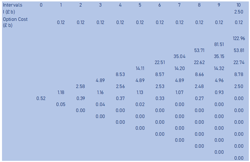
From the above event tree, we now have the option value at year 0 and we can now calculate the expanded NPV of the opportunity.
Step 5. Option Value and Expanded NPV
Based on the final pay-off binomial event tree, we get an option value of £0.52billion. From this we can now calculate the expanded NPV using the formulae
Expanded NPV = Static NPV + Option Value
= -£0.2 billion + £0.52 billion
= £ 0.32 billion
So by taking an option to delay and learning more about the true nature of the opportunity, Qubixz Limited is able to launch its wearable device and capture value of up to £320 million, compared to the negative £200 million predicted by the traditional NPV.
It is worth noting that to maintain a positive value on the wearable innovation opportunity, the total cost of patent, any market research and prototyping during the life of the option (cost that are not considered in the above analysis) must not exceed £320 million.
The above example considers exercising the option at year 10. If Qubixz wants to exercise the option earlier (say at the end of year 7, then the option will be framed up to the year of exercise (year 7) rather than up till year 10. In this scenario, the pay-offs will be calculated using value of V at year 7, then the same discounting back to year zero will be performed to get the option value.
Option to Expand Case Study
Qubixz UK Limited is launching a new fitness-as-a-service business within the square mile in London. Whilst the new service shows that an Investment of £1.55m will only return a present value of cash flow of £1m, this initial investment will position Qubixz to be able to rapidly expand the service throughout the rest of London over the next five years. If Qubixz expands throughout London the venture will cost £25m in capital investment, with initial estimate of cash flows over 20 years providing a present value of £21 m. Despite this seemingly unattractive numbers, Qubixz understands that standard deviation in firm values for the fitness industry is a significant 60.96%. As such Qubixz is convinced that an option to expand will turn the initial investment into a strategic one. Based on current analysis, the following data has been generated
Cost of launching service in square mile, I = £ 1.55 m
PV of cash flow in square mile, V0= £ 1 m
Cost of expanding service throughout London, Ie = £ 25 m
PV of cash flow after expansion, V0e= £ 21 m
Period in which Qubixz can expand (option life), t = 5 years
Risk free rate, r = 2% (5 year UK govt. treasury rate)
Volatility expected in value, s = 0.61 (This is SD in firm value in fitness industry)
cost per year, c = (21/20) = £1.05 m/yr
We will now take a stepwise approach to valuing the option to expand this investment and the resulting expanded NPV
Step 1. Traditional NPV Calculation
First we look at the static NPV of this opportunity, which considers investing in the service based on Cost of Investment and PV of cash flows. We get an NPV of -£ 0.55m (£1m - £1.55m), thus making this a non-viable standalone project (today) from the NPV point of view.
However, as we know, this initial loss making investment is a strategic one to position Qubixz for potential growth.
Step 2. Build the Event Tree of Future Values
To assess the option to expand at the 5 year expiration and see if there is a chance that the option value will result in opportunity being economically viable, we need to build an event tree of future values.
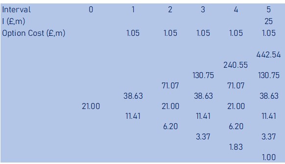
To do this, based on the volatility we will determine how the expansion asset value of £21m may grow or diminish over the next 5 years. For this we need to calculate the u and d factors. Using yearly intervals (5 intervals), we calculate as follows
u = exp (s*√dt) = exp (0.61*sqrt (5/5)) = 1.84
d = 1/1.84 = 0.54
Based on the PV of cash flow and the u and d factors, we can now build our binomial event tree of all the possible future values of the expansion opportunity over the next 5 years. As an example, the first up value and down value are calculated as
21*1.84 = £38.63 m
21*0.54 = £11.41 m
Possible future asset values (V, £ million) of Qubixz Limited’s new fitness-as-a-service is as shown in the binomial tree below
Step 3. Determine the Pay-off at Option Exercise
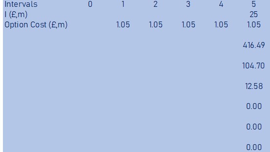
From the future values (V), we will now calculate all the possible pay-offs during expansion option exercise at the end of the option life (year 5). The pay-off will be the Maximum (V – I – c , 0).
As an example, for V at the top right hand corner of the tree, which shows that if the value of the asset went up every year it will reach £442.54m, the pay-off will be
442.54 – 25 – 1.05 = £ 416.49m
Whilst at the bottom right hand corner of the tree, which shows that if the value of the opportunity went down every year it will fall to £ 1m, the pay-off will be
1 – 25 – 1.05 = £ 0
The implication here is that, for future values that have a positive pay-off, logically Qubixz Limited will most likely choose to exercise this option and expand and for future values that have a negative pay-off, Qubixz Limited will not exercise its option to expand, making the pay-off zero.
Using this Max pay-off calculation formulae, we will calculate the pay-off for all future values V at the final year of the option, which is year 5 in this case. The result is shown in the binomial tree year 5 pay-offs table below.
The next step is to then discount these pay-offs back to time zero.
4. Discount Pay-offs Back to Year 0
Once we determine all pay-off values at year 5 where Qubixz Limited may choose to exercise the option to abandon this venture, we will now discount all the pay-offs back to the present using the risk free discount rate and probabilities of both u and d movements.
pu = [exp(0.02*1)-0.54]/[1.84-0.54] = 0.368
pd = 1 - pu = 0.632
As an example, discounted values of the top two pay-offs from year 5 to year 4 minus the forgone minimum income in year 4, will be as shown below
(416.5*0.368 + 104.7*0.632) / (1.02) – 1.05 = £ 215.1m
Similarly, discounting the bottom two values from 5th year to 4th year will be as shown below
(0*0.368 + 0*0.632) / (1.02) – 1.05 = £ 0
This exercise is carried out from the 5th year pay-off values, back one year at a time, such that the values calculated for year 4 are used to determine the values in year 3, all the way till year zero.
This exercise will give the below binomial event tree
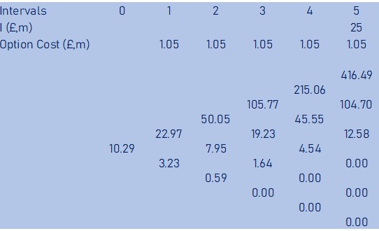
From the above event tree, we now have the option value at year 0 and we can now calculate the expanded NPV of the option to abandon.
Step 5. Option Value and Expanded NPV
Based on the final pay-off binomial event tree, we get an option value of £10.3m. From this we can now calculate the expanded NPV including option to expand using the formulae
Expanded NPV = Static NPV + Option Value
= -£0.55m + £10.3m
= £ 9.74m
So by having an option to expand that provides a positive Expanded NPV despite the negative value of the initial investment, Qubixz Limited is able to launch its fitness-as-a-service in the square mile and if the market proves to follow the upside of the real option valuation, then Qubixz will expand across London. If the market follows the downside, Qubixz will walk away from its option to expand. In this option to expand, the £0.55m is equivalent to a call option price and will represent the maximum downside if Qubixz is not able to take the option to expand. Note that for option to expand, we only consider the expansion option value since Qubixz will only expand if the outcome of the market is positive during the initial investment and option life, if the outcome is negative Qubixz will walk away and will thus not incur the negative static NPV calculated for the expansion case.
It should also be noted that there are cases where the option value will result in an Expanded NPV that is still negative. In that case, Qubixz is unlikely to proceed with the initial investment, since if the market conditions turns out positive the follow on investment doesn’t have high enough option value to turn the overall venture around.
Option to Abandon Case Study
Qubixz UK Limited is working on producing and installing new super-fast charging stations for electric vehicles across the UK. Due to the rapidly emerging EV market, Qubixz is not looking at an option to delay despite the initial negative static NPV (see below). Qubixz is planning to proceed, since volatility means the negative NPV may still turn positive in a few years. Despite this and as an insurance policy, Qubixz wants to evaluate the option to abandon the project in case the venture really does turn out disappointing. Qubixz has analysed that the real estate of where the charging stations will be installed can be sold for £80m within 5 years and the charging equipment across all stations will have a resell value of £120m, also within 5 years. Based on current analysis, the following data has been generated
Cost of developing the charging stations, I = £ 350 m
PV of 30 year cash flow if charging stations are launched now, V0= £ 300 m
Total Asset (land + charging equipment) Recovery Value, R = £200 m
Other expenses for Abandonment, Ae = £5m
Period in which cost can be re-couped (option life), t = 5 years
Risk free rate, r = 2% (5 year UK govt. treasury rate)
Volatility expected in value, s = 0.35 (This is SD in firm value in Auto industry)
Income per year, i = (300/30) = £10 m/yr
We will now take a stepwise approach to valuing the option to delay this investment and the resulting expanded NPV
Step 1. Traditional NPV Calculation
First we look at the static NPV of this opportunity, which considers investing in the project based on Cost of Investment and PV of cash flows. We get an NPV of -£ 50 million, thus making this a non-viable project (today) from the NPV point of view.
Step 2. Build the Event Tree of Future Values
To assess the option to abandon, based on the asset recovery value and in the event that the upside of the volatility doesn’t materialise and Qubixz may need to walk away to avoid a return of negative £ 50million or worse we need to build an event tree of future values relating to abandonment.
It should be noted that an option to abandon (which is synonymous to put option) is different to option to delay (synonymous to a call option). Consequently, rather than incur cost leading up to the option exercise, here Qubixz Limited will take into account the revenues estimated in the 5 years leading up to the option exercise (since the venture has already gone ahead in this case), which in this case is £10m per year (300/30). Additionally, the value of asset used to start the binomial tree will not be V0, instead it will be the outstanding asset value of the estimated V0 that will be forgone when the option to abandon is exercised, which is £250m (300 – 10*5).
Based on the above and based on calculated values of u (1.419) and d (0.705), the binomial tree of future values is as shown below
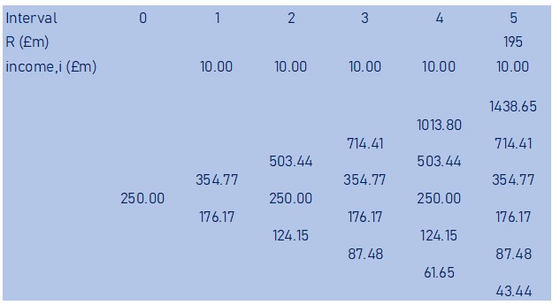
Step 3. Determine the Pay-off at Option Exercise
From the future values (V), we will now calculate all the possible pay-offs during abandon option exercise at the end of the option life (year 5). The pay-off will be the Maximum (R – Ae + i – V, 0).
As an example, for V at the top right hand corner of the tree, which shows that if the value of the asset went up every year it will reach £1439m, the pay-off will be
195 + 10 – 1439 = £ 0
Whilst at the bottom right hand corner of the tree, which shows that if the value of the opportunity went down every year it will fall to £ 43m, the pay-off will be
195 + 10 – 43 = £ 162m
Note that the pay-off is the recovery value less any expenses incurred as part of the abandonment exercise. Here this is a £5m expense to abandon the project. This could be settle of staff or government fees etc. Hence the net recovery here is £195m (200 – 5).
The implication here is that, for future values that have a positive pay-off, logically Qubixz Limited will choose to exercise this option and abandon its EV charging venture (since the value of income from recovery plus that years’ income exceeds the value of the venture) and for future values that have a negative pay-off (EV charging is proving economically viable), Qubixz Limited will not exercise its option to abandon (since the value of income from recovery plus that years’ income is less than the value of the venture) making the pay-off zero.
Using this Max pay-off calculation formulae, we will calculate the pay-off for all future values V at the final year of the option, which is year 5 in this case. The result is shown in the binomial tree year 5 pay-offs table below.
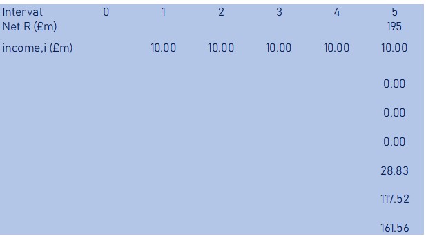
The next step is to then discount these pay-offs back to time zero.
4. Discount Pay-offs Back to Year 0
Once we determine all pay-off values at year 5 where Qubixz Limited may choose to exercise the option to abandon this venture, we will now discount all the pay-offs back to the present using the risk free discount rate and probabilities of both u and d movements.
pu = [exp(0.02*1)-0.705]/[1.419-0.705] = 0.442
pd = 1 - pu = 0.558
As an example, discounted values of the bottom two pay-offs from year 5 to year 4 plus the year 4 income from the venture, will be as shown below
(118*0.442 + 162*0.558) / (1.02) + 10 = £ 149m
Similarly, discounting the top two values from 5th year to 4th year will be as shown below
(0*0.442 + 0*0.558) / (1.02) + 10 = £ 10m
This exercise is carried out from the 5th year pay-off values, back one year at a time, such that the values calculated for year 4 are used to determine the values in year 3, all the way till year zero.
This exercise will give the below binomial event tree
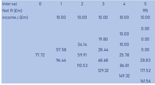
From the above event tree, we now have the option value at year 0 and we can now calculate the expanded NPV of the option to abandon.
Step 5. Option Value and Expanded NPV
Based on the final pay-off binomial event tree, we get an option value of £80m. From this we can now calculate the expanded NPV including option to abandon using the formulae
Expanded NPV = Static NPV + Option Value
= -£50m + £78m
= £ 28m
So by having an option to abandon that proves a positive Expanded NPV despite the negative value of the traditional NPV, Qubixz Limited is able to launch its EV charging station in the knowledge that if volatility works in its favour, the venture can be continued, otherwise Qubixz can exercise the option to abandon within 5 years and still end up in a positive NPV.
Concluding Remarks
Within this article, we have demonstrated that real options valuation can add value on top of the traditional NPV to provide an expanded and more complete value creation potential of an innovation opportunity. This is critical in eliminating two types of errors – investing in opportunities that are not economically viable and rejecting investment in opportunities that are highly economically viable. When innovations are structured as real options, this in effect places a value on uncertainty (risk) and flexibility, enabling the organisation to exercise the option to capture the value from the risk upside whilst being able to walk away from the downside. This is a key and critical feature, as these risks (both upside and downside) are discounted as having negative impact on economic value (based on risk adjusted WACC in discounted cash flow) when the traditional NPV approach is taken.
Despite its benefits, the adoption of real options valuations remains relatively low. This is in part due to any combination of the three following factors; lack of awareness, complexity of methodology and scepticism with regards to over-valuation of opportunities.
We hope that this article will help to further raise awareness on real options valuation and the binomial pricing model used offers an easier to comprehend methodology. With regards to scepticism of overvaluation, which is argued to stem from lack of exclusivity on market opportunities and can reduce the option value below the estimate, we note the following. Whilst we agree that full exclusivity is the ideal scenario, this concern is not specific to real options but also applicable to the traditional NPV. A key input factor for real option valuation is the asset value (which is PV of all post tax cash flows). This asset value is a key component in the NPV methodology and is typically based on an assumption that a certain percentage of the market (or a certain number of customers will be captured by the company). As such, by using the same present value of cash flow, real options valuation does not deviate from the original assumption, hence the concern over lack of exclusivity (for opportunities where there is no patent protection or guaranteed customer base due to excess demand) is a universal one, rather than specific to real options methodology.
In conclusion, to ensure innovating organisations are positioned to capture the upside of uncertainty and risk of innovation and reject the downside, innovation leaders must adopt real options valuation as a key component of their innovation management process. Real options will help such organisations to reveal the value that lies beyond traditional NPV.
If you have any queries on this article or on adoption or implementation of real options valuation, contact us at enquiry@innstrat.com